Getting Started
A simple example of running a structural simulation using the Intact CLI. This guide walks through the JSON structure needed to define a cantilever beam simulation.
Typical Workflow
Set up the input JSON and provide the geometry file (.VDB, .PLY, .STL) and boundary condition faces (.STL, .PLY)
Execute intact CLI:
$ intact -s "path to json file" --save-solution --refinement-level 0.02A successful run will result in a
*_samples.vturesult fileYou can visualize the result in Paraview (an open source program, see instructions below)
Resample the saved solution on a new geometry (sections or cuts)
Modify geometry file in the original JSON to the new geometry that you want to resample on
Execute:
$ intact -s "path to json file" --load-solution-file --refinement-level 0.02
JSON Structure
An Intact CLI simulation is defined by a JSON file that brings together all the components of your analysis. The JSON file has the following main sections:
{
  "type": "LinearElasticity",
  "scenario_name": "my_simulation",
  "geometry": { },
  "materials": { },
  "boundary_conditions": [ ],
  "internal_conditions": [ ],
  "metadata": { }
}
Main Sections:
type: Specifies the physics type for the simulation (e.g.,"LinearElasticity","Modal","LinearBuckling","StaticThermal","ThermoLinearElasticity"). See How To: Metadata and Physics Types for details on each physics type.scenario_name: A descriptive name for your simulation.geometry: Defines the geometric model including components and assembly. See How To: Units, Geometry, and Materials for detailed geometry specification.materials: Specifies material properties (isotropic, orthotropic, or thermal materials). See How To: Units, Geometry, and Materials for material definitions.boundary_conditions: Array of boundary conditions applied to surfaces (restraints, loads, thermal conditions). See How To: Boundary Conditions for all available boundary condition types.internal_conditions: Array of internal conditions applied to volumes (body loads, rotational loads, heat generation). See How To: Internal Conditions for details.metadata: Solver parameters and configuration options (resolution, units, solver type, etc.). See How To: Metadata and Physics Types for all metadata options.
The following sections provide a simple example of each component to get you started.
Create Geometry
Geometry is specified in the geometry object, which contains two parts: components and assembly.
{
  "geometry": {
    "components": [
      {
        "file": "beam.stl",
        "geometry_type": "Mesh",
        "id": 0,
        "material": "steel"
      }
    ],
    "assembly": [
      {
        "component": 0,
        "instance_id": "simple_cantilever",
        "type": "Component"
      }
    ]
  }
}
Create Material
Materials are defined in the materials object. Each material must specify a type and relevant properties.
{
  "materials": {
    "steel": {
      "type": "Isotropic",
      "failure_criterion": "VonMises",
      "density": 7800.0,
      "youngs_modulus": 2.1e11,
      "poisson_ratio": 0.3,
      "yield_strength": 330000000.0,
      "tensile_strength": 0.0,
      "compressive_strength": 0.0
    }
  }
}
Create Boundary Conditions
Boundary conditions are specified in the boundary_conditions array. Each boundary condition requires a type and a boundary surface file.
{
  "boundary_conditions": [
    {
      "boundary": "fixed_face.ply",
      "type": "fixed"
    },
    {
      "boundary": "load_face.ply",
      "type": "vector_force",
      "direction": [0, -1, 0],
      "magnitude": 1000,
      "units": "MeterKilogramSecond"
    }
  ]
}
Setup Simulation
Finally, specify the metadata to control solver parameters:
{
  "metadata": {
    "resolution": 10000,
    "units": "MeterKilogramSecond"
  }
}
Complete Example
A complete cantilever beam simulation example is available for download:
More Examples
Demo examples with both Mesh and VDB geometry are available for download:
These examples demonstrate various simulation types and boundary conditions.
Viewing Results
The intact command line outputs VTK files. These are fairly standard, and can be manipulated in a variety of programming languages. For more information about official VTK resources please check out their homepage.
VTK - The Visualization Toolkit
There are a number of third-party libraries for working with VTK files in other languages.
We recommend using the Paraview application for viewing and manipulating these results in most cases. Paraview is an industry-standard scientific data analysis and visualization tool that is free and open-source. More information, and builds for most operating systems, are available from the Paraview home page.
Paraview Quick-start
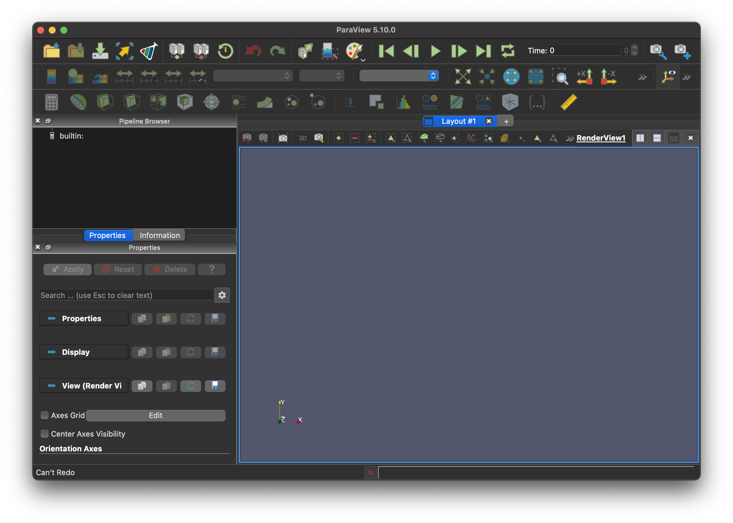
Opening Paraview should yield an interface that looks roughly like this.
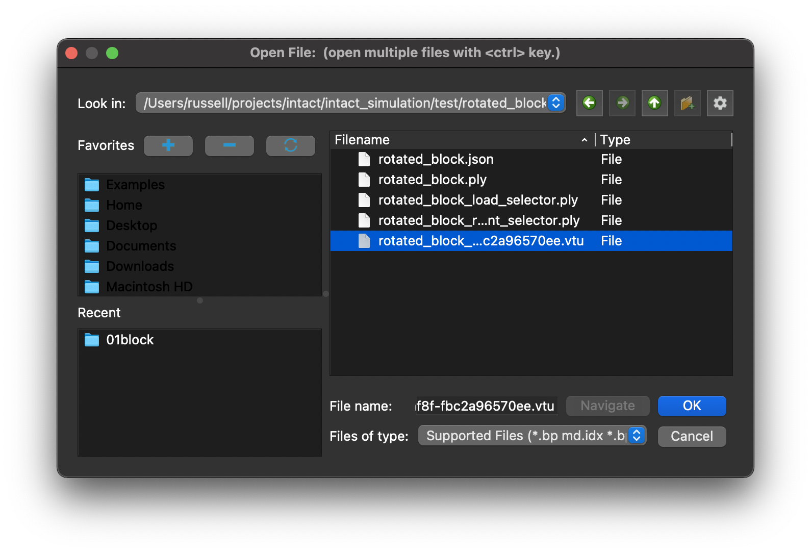
The intact command line tool will place the samples in the results directory (by default, the same directory as the json file). Look for a samples *.vtu file and open it in Paraview.
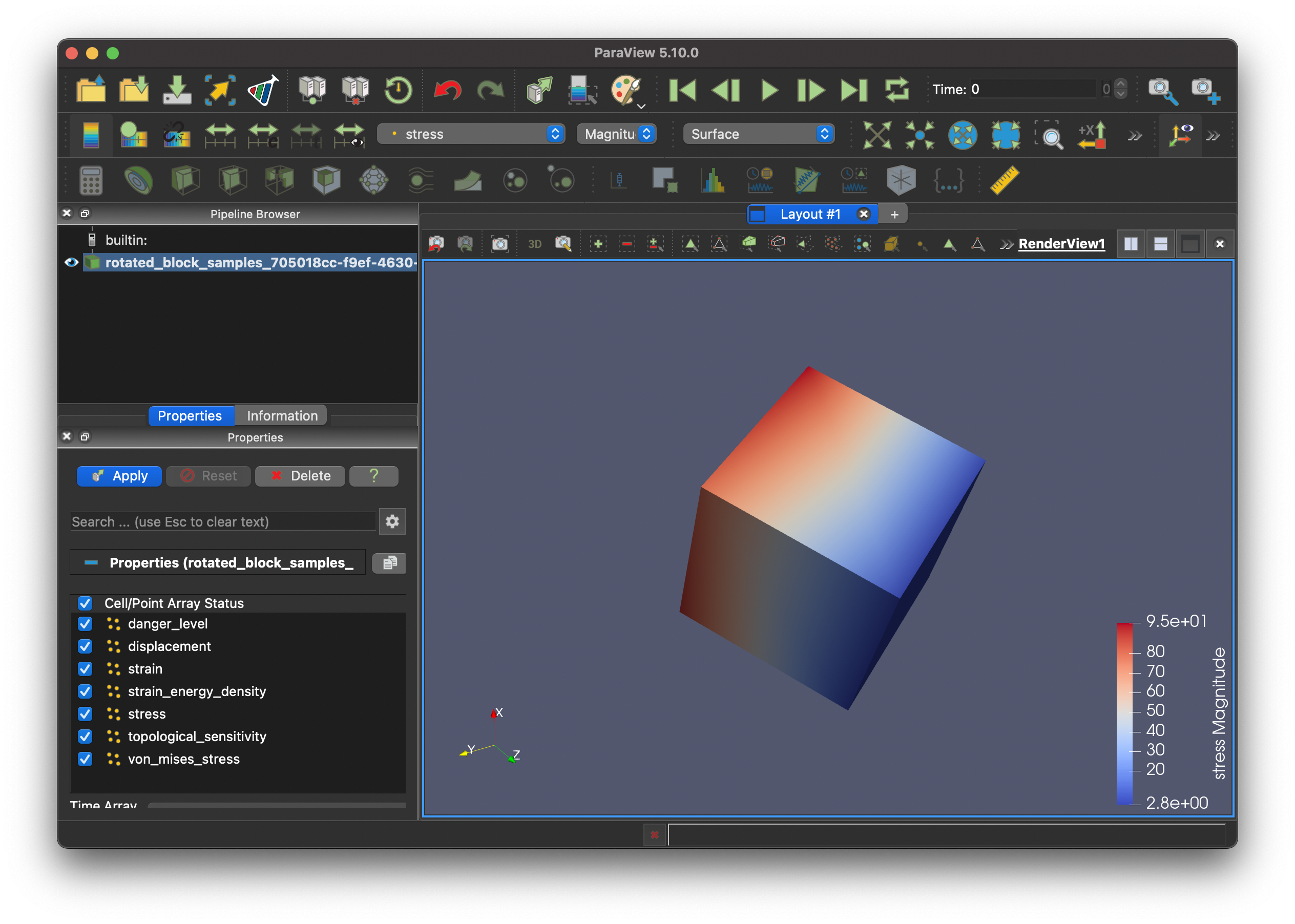
Make sure the samples are visible in the pipeline browser by clicking the eye icon.

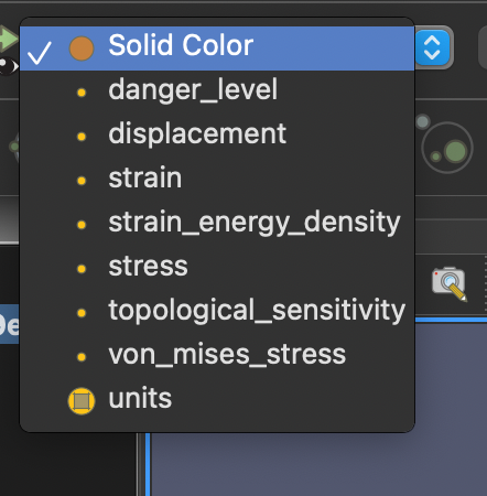
The sampled fields are available in the properties dropdown. For example the following would be typical of a linear elasticity scenario.
Here is how stress results would look. One can rotate and pan the viewport.