Intact CLI 1.0.19 User’s Manual
Introduction
The Intact command line tool allows users to run a variety of physics simulations over assemblies of different geometry types. These simulations are configured with a json file. We generally refer to one of these simulations as a scenario. Code examples that are meant to be run in a shell are prefixed with $. For example
$ intact --help
will produce output that looks like:
$ intact --help
A command line interface for Intact
For more information, the user manual can be found at:
https://intact-solutions.com/intact_docs/
Usage:
  Intact [OPTION...]

  -h, --help                    Print program usage
      --build-info              Print report about current build, then exit
      --version                 Print the software version
  -s, --scenario arg            Scenario json file
  -f, --fields arg              Fields to sample (if empty, all available
                                fields will be sampled). Comma delimited.
  -o, --output arg              Output directory. The default it the
                                directory of the scenario file.
      --skip-sample             Skip the sampling step of the solver.
      --json-output             Output the sampled results in JSON format
                                (VTK is the default output).
      --tempdir                 Make a temporary directory for output
      --scenario-name arg       Prefix for output files, defaults to
                                scenario file name
      --load-solution-file      Load a cached solution file/s
      --logdir arg              Path to the log file. Default value is
                                current working directory.
      --logname arg              If not specified, log will not be put in a
                                file
      --save-solution           Save the scenario solution in vtk format
      --refinement-level arg    Refinement ratio w.r.t. assembly bounding
                                box. If not present, no refinement is
                                performed.
  -v, --verbosity arg           Verbosity level, run with --help for more
                                information
      --define-version          Software version
Aside from the syntax for paths, this documentation applies to builds of the intact tool on all operating systems. All officially supported features are documented here, though the build provided may have additional functionality.
In addition, this manual should be bundled with example simulation files. We advise looking at those as a companion to the material described here.
Example Simulation to Get Started
Instructions
Sign up for the trial to get access to our software.
The intact CLI executable is installed in C:\Users[your username]\AppData\Local\Programs\Intact.Simulation for Automation\intact.exe
Some demo examples (Mesh and VDB geometry).
Typical workflow
Set up the input Json and provide the geometry file (.VDB, .PLY, .STL) and boundary condition faces (.STL, .PLY)
Execute intact CLI $ intact -s “path to json file” –-save-solution –refinement-level 0.02
A successful run will result into a *_samples.vtu result file
You can visualize the result in Paraview (an opensource program, see instruction below)
Resample the saved solution on a new geometry (sections or cuts)
Modify geometry file in the original JSON to the new geometry that you want to resample on
Execute $ intact -s “path to json file” –load-solution-file –refinement-level 0.02
Viewing Results
The intact command line outputs VTK files. These are fairly standard, and can be manipulated in a variety of programming languages. For more information about official VTK resources please check out their homepage.
VTK - The Visualization Toolkit
There are a number of third-party libraries for working with VTK files in other languages.
We recommend using the Paraview application for viewing and manipulating these results in most cases. Paraview is an industry-standard scientific data analysis and visualization tool that is free and open-source. More information, and builds for most operating systems, are available from the Paraview home page.
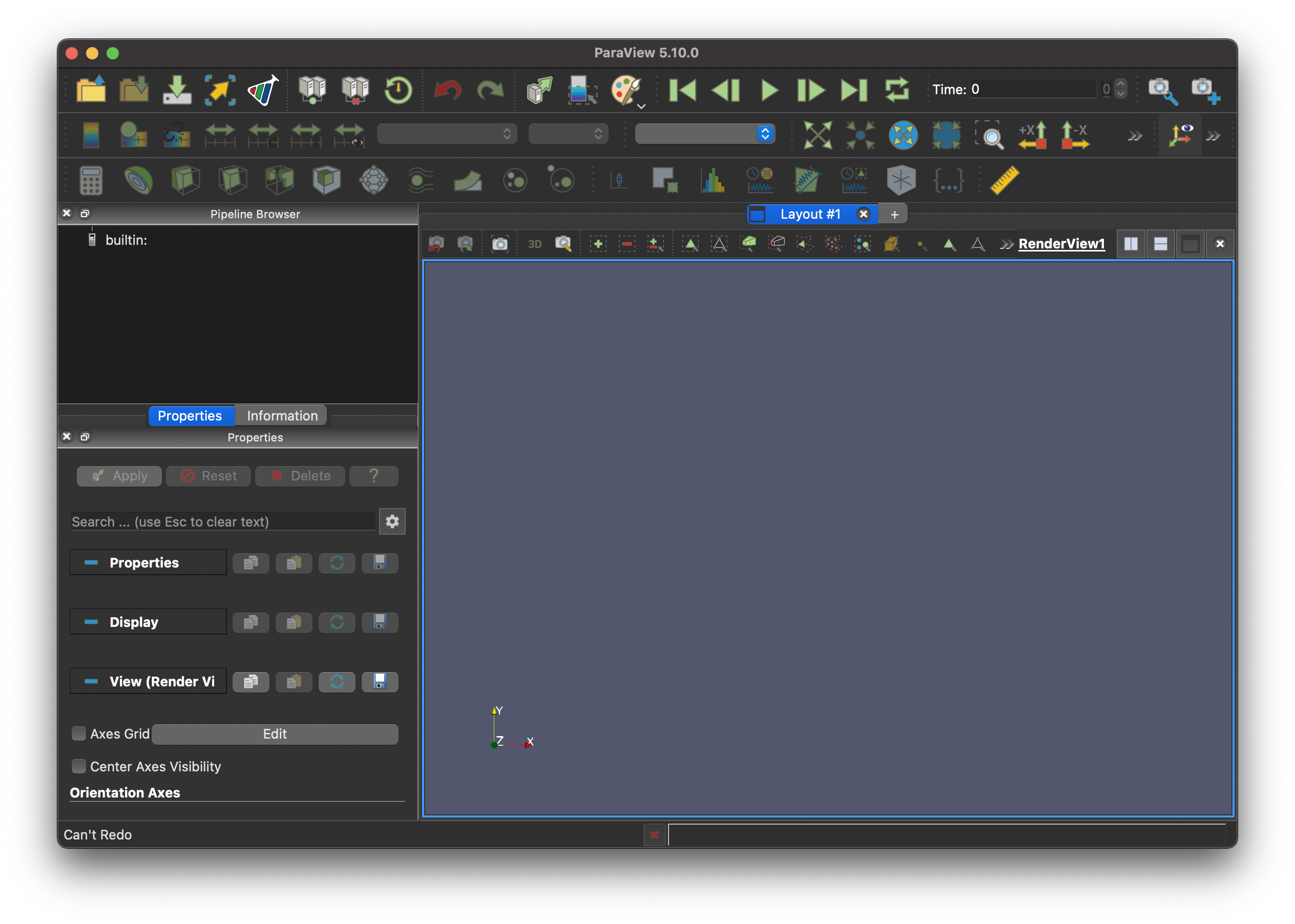
Paraview Quick-start
Opening Paraview should yield an interface that looks roughly like this.
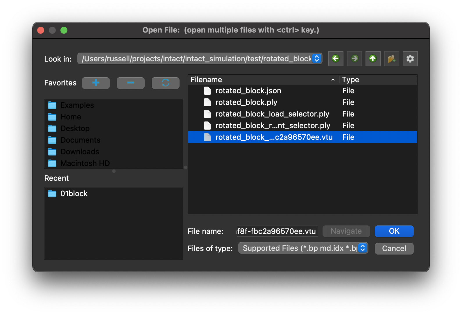
The intact command line tool will place the samples in the results directory (by default, the same directory as the json file). Look for a samples *.vtu file and open it in Paraview.
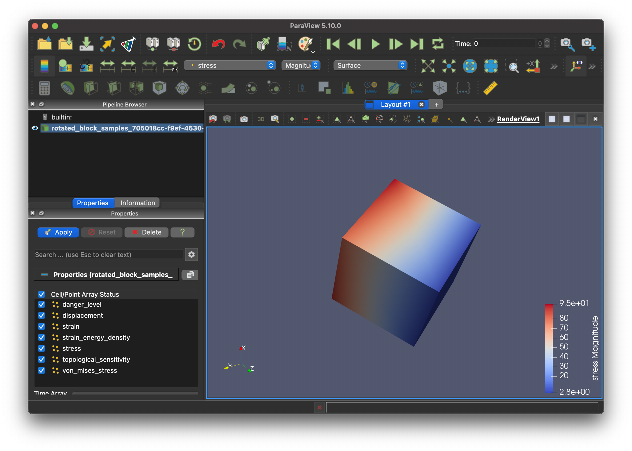
Make sure the samples are visible in the pipeline browser by clicking the eye icon.

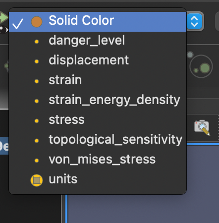
The sampled fields are available in the properties dropdown. For example the following would be typical of a linear elasticity scenario.
Here is how stress results would look. One can rotate and pan the viewport.
Command Line Options
Command line documentation can be retrieved with the help flag.
$ intact --help
The help documentation bundled with the tool is definitive, the most important options are covered here in more detail.
-s, --scenario <path/to/scenario.json>
When not calling either --help or --build-info, this option is mandatory for all calls. The tool needs a path for the scenario json file to use.
-o, --output <path/to/output_dir>
The tool generates a variety of output files. By default, these files will be put in the same directory as the scenario json file. Use this flag to change the directory where output files will be placed. The scenario json file, and any geometry files referenced, will be copied over to the output directory.
--refinement-level <ratio>
Surface and Volume mesh geometry can be refined prior to sampling. This can be a good idea if the triangle quality is poor: large triangles may not properly resolve and interpolate detail in the solution. Refining the mesh means that the ratio of element edge length to bounding box size will not exceed the refinement level provided by this option.
--build-info
This flag can be used to get detailed information about the version of the tool. Attaching this information to any bug reports will help with debugging.
Specifying Boundary Conditions
Specifying boundary conditions for Intact.Simulation is a bit different than other FEA systems. Because Intact’s technology is based on the use of a non-conforming mesh, boundary conditions are not specified directly on a finite element mesh. This also means that Intact does not support non-real boundary conditions like point and edge constraints / forces / moments.
Instead, boundary conditions in Intact are specified as triangle mesh based surfaces. These can be either *.ply or *.stl files. Specific semantics of what each boundary conditions does are specified in the section for each physics, however all boundary conditions will need to specify a surface.
Some things to keep in mind with these surfaces.
Having multiple disconnected components in one mesh will not cause a runtime error but may not yield high quality results. It is best to create a separate boundary condition instance in the json configuration for each fully connected component.
It is possible to specify a boundary condition that is disconnected from the geometry. This can result in a runtime warning, but is not an error. Note in cases where a force / quantity is distributed over the boundary condition surface this will result in some of the quantity not being accounted for since there is nothing to apply it to.
Common JSON Keys
The scenario json format shares a lot of structure between the different physics. The common components are detailed here. All scenario json files start with a top-level object, which contains a few common attributes.
{
  "boundary_conditions": [ ... ],
  "geometry": { ... },
  "materials": { ... },
  "metadata": { ... },
  "scenario_name": "Name_for_output_files",
  "type": "<physics type>"
}
Geometry
Specifying geometry in scenario json has two pieces. First, a collection of components must be defined. Each component has a geometry type, a file to load, a material id, and a component id. The other component to specifying geometry is an assembly of components. The material id needs to match a material defined in the materials object from the scenario object. Each component needs a unique integer id.
Geometry::Mesh
There are four types of geometry that can be used with components. The most common is to use a triangle mesh to specify the surface of a volume. These triangle meshes can be loaded from both ply and stl files.
{
  "file": "block.ply",
  "geometry_type": "Mesh",
  "id": 1,
  "material": "Acrylic"
}
Geometry::VDB
Geometry can be specified with an openvdb double grid file.
{
  "file": "demo.vdb",
  "geometry_type": "VDB",
  "id": 2,
  "material": "Steel"
}
Units
There are several places in the json format where units can be specified. The possible values are listed here.
"MeterKilogramSecond"
"CentimeterGramSecond"
"MillimeterMegagramSecond"
"FootPoundSecond"
"InchPoundSecond"
Boundary Conditions
All scenarios require the specification of boundary conditions. Different scenarios support different types of boundary conditions, but all boundary conditions have a couple of common members.
boundary
All boundary conditions must be applied to a specified surface. The value should be a path to an *.ply or *.stl file. This path can be relative to the location of the scenario json file. For example, if the configuration json file is in the same directory as restraint.ply then the following would be valid.
"boundary": "restraint.ply"
units
All boundary conditions can optionally specify units.
type
The type member differentiates the variety of possible boundary conditions. Each specific boundary condition will contain an example json instance that will have the value for type.
Metadata
There are a variety of options available that can be configured with metadata.
Either resolution or cell_size must be specified, but no other options need to specified.
Default values will be used when not specified.
units
The default units for the scenario, including geometry. Note that this default does not apply to materials, which will default to MKS unless specified there.
basis_order
The type of finite element used. The default is 1, which would be linear elements. 2 is for quadratic elements.
max_iterations_multiplier
This parameters changes the max iterations for iterative solvers, it scales with the number of degrees of freedom. Use a parameter less then one for faster solve times, with the tradeoff of accuracy.
tolerance
The tolerance for iterative solvers. The default value is 1e-20. That value is meant to achieve high accuracy at the cost of solve runtime. Increasing the tolerance will decrease solve time, but will yield less accurate results.
resolution
The target number of elements. An iterative process is used to determine a cell size that achieves approximately the specified number of elements. The logging output will include the resolved number of elements and cell size. Either resolution or cell_size must be specified.
cell_size
The cell size to use. The log output will include the resolved number of elements. When possible, specifying cell_size will skip the expensive iterative process when using the resolution parameters.
omega_cutoff
A parameter to tune the use of solution structure method for enforcing boundary conditions. By default, there is no cutoff, and it is not recommended to tune this parameter without additional input from Intact Solutions.
solver_override
The solver_override parameter can be used to explicitly specify the solver to use.
The default solver for linear elasticity and modal scenarios is AMGCL_amg_rigid_body.
The default solver for thermal scenarios is AMGCL_amg.
The following solvers are available:
  // Iterative conjugate gradient solver without preconditioner.
  AMGCL_cg

  // Iterative conjugate gradient solver with ilu0 preconditioner.
  AMGCL_ilu0_cg

  // Iterative conjugate gradient solver with damped jacobi predonditioner.
  AMGCL_damped_jacobi_cg

  // Iterative AMG based solver with smoothed aggregation.
  // This is the default solver for thermal scenarios.
  AMGCL_amg

  // Iterative AMG based solver with rigid body modes based coarsening.
  // This is the default solver for linear elasticity.
  // This solver cannot be used with thermal scenarios.
  AMGCL_amg_rigid_body

  // Direct solver that uses LU decomposition.
  Eigen_SparseLU

  // A sparse direct Cholesky (LDLT) factorization and solver based on the PARDISO library provided by Intel's MKL.
  MKL_PardisoLDLT

  // A sparse direct Cholesky (LLT) factorization and solver based on the PARDISO library provided by Intel's MKL.
  MKL_PardisoLLT

  // A sparse direct LU factorization and solver based on the PARDISO library provided by Intel's MKL.
  MKL_PardisoLU
integrator_override
For some physics types, there may be multiple integrator implementations available;
the integrator_override configuration allows choosing among the available implementations.
In general, the default choice is the best choice.
The following integrators are available:
  // Default for modal scenarios.
  IntactModal

  IntactLinearElasticity

  // Default for thermal scenarios.
  MPCStaticThermal

  // Default for linear elasticity scenarios.
  MPCLinearElasticity

  LinearBuckling
use_caching
By default, Intact.simulation will cache all quadrature rules and material properties for each cell. This can use significant amounts of memory for problems with lots of elements. To really push the problem size that can be run on a given machine, caching can be turned off to decrease the memory footprint of a simulation run at the cost of additional runtime.
"use_caching": false
verbose_solver
Some of the sparse linear solvers used by intact can provide feedback about their progress. By default this is false, but if set to true some solvers will report their progress to standard out. For AMGCL solvers, every five iterations the iteration number and various error measurements will be printed. This can be useful for long running simulations to observe progress.
Linear Elasticity
Linear elasticity requires the scenario json object to have "type": "LinearElasticity".
Materials
Linear Elasticity and Modal scenarios both use our structural material types. All materials need a density value, and can optionally include a "units": member. Note that all materials will be specified in MKS unless units are specified.
Isotropic
For isotropic materials, the user must specify a failure criterion type. This is used during sampling to calculate the topological sensitivity and danger level, fields which aren’t sampled for other structural material types. The choices for failure criterion type are:
"Unspecified" // Do not calculate the danger level
"VonMises"
"MaximumShearStress"
"Rankine"
"CoulombMohr"
"ModifiedMohr"
An example of how this would look in json:
{
  "compressive_strength": 690000000.0,
  "density": 7200.0,
  "failure_criterion": "CoulombMohr",
  "poisson_ratio": 0.27,
  "tensile_strength": 170000000.0,
  "yield_strength": 0.0,
  "youngs_modulus": 100000000000.0
}
Orthotropic
Orthotropic materials have material properties that vary depending on the orientation.
The elastic modulus in the x, y and z directions are defined by Ex, Ey and Ez,
the Poisson’s ratio by vxy, vxz and vyz,
and the shear modulus by Gxy, Gxz and Gyz.
The material properties can be transformed by specifying a transform matrix, for example,
to simulate composite fibers that are rotated by 45° relative to the x-axis.
The type must be Orthotropic.
An example configuration for a composite material of Kevlar and epoxy, with the fibers rotated by 45° relative to the x-axis, is shown below.
{
  "Ex": 85000000000.0,
  "Ey": 5600000000.0,
  "Ez": 5600000000.0,
  "Gxy": 2100000000.0,
  "Gxz": 2100000000.0,
  "Gyz": 2280000000.0,
  "density": 1350,
  "transform":
    [0, 0.7071, 0.7071,
     0, -0.7071, 0.7071,
     1, 0, 0],
  "vxy": 0.34,
  "vxz": 0.23,
  "vyz": 0.34,
  "type": "Orthotropic"
}
Boundary Conditions
Fixed
Fixes the boundary at 0.
Fixed boundary conditions can be applied to both thermal and displacement fields.
Fixed displacement boundary conditions are often called restraints in other FEA systems.
{
  "boundary": "restraint_selector.ply",
  "type": "fixed"
}
For thermal scenarios, temperature fields can be fixed to non-zero values with the optional value field.
{
  "boundary": "restraint_selector.ply",
  "type": "fixed",
  "units": "FootPoundSecond",
  "value": 500.0
}
Fixed Vector
This boundary condition serves two purposes.
Fixing displacement at some non-zero value.
Partial restraints, also known as axis-aligned sliding restraints.
Displacement is a three dimensional field, and each displacement component can optionally be specified. Any axis not specified will not be restrained. The following example fixes the x component of displacement at 1, while the y and z axis are unrestrained.
{
  "boundary": "restraint_selector.ply",
  "type": "fixed_vector",
  "units": "MillimeterMegagramSecond",
  "x_value": 1.0
}
In the following example, the x axis is fixed at 1.0, while the y and z axis are fixed at 0.
{
  "boundary": "restraint_selector.ply",
  "type": "fixed_vector",
  "units": "MillimeterMegagramSecond",
  "x_value": 1.0,
  "y_value": 0.0,
  "z_value": 0.0
}
Sliding
Sliding boundary conditions prevent displacement in the direction normal to the specified surface, and permit displacement tangential to the surface. A sliding boundary condition can be used to represent a pin joint, for example.
To use a sliding boundary condition, specify the boundary where this boundary condition applies,
and specify the type as sliding, as in the following example:
{
  "boundary": "restraint_selector.ply",
  "type": "sliding"
}
Vector Force
The vector force boundary conditions will apply a force of a given direction and magnitude evenly over the prescribed surface. Vector force must specify the direction and magnitude.
{
  "boundary": "surface.ply",
  "direction": [
    0.0,
    0.0,
    -1.0
  ],
  "magnitude": 100.0,
  "type": "vector_force",
  "units": "MillimeterMegagramSecond"
}
Pressure Force
A pressure force boundary condition applies a pressure of a given magnitude opposing the normal of the boundary.
{
  "boundary": "top_face.ply",
  "magnitude": 100.0,
  "type": "pressure_force",
  "units": "InchPoundSecond"
}
Torque Force
Applies a torque force to the boundary. Must specify the axis and origin of the rotation, as well as the magnitude of the torque.
{
  "axis": [
    0.0,
    0.0,
    1.0
  ],
  "boundary": "twist_load_selector.ply",
  "magnitude": 100.0,
  "origin": [
    0.0,
    0.0,
    20.0
  ],
  "type": "torque_force"
}
Hydrostatic Load
A hydrostatic load boundary condition simulates a body submerged in liquid,
and requires defining the boundary that may be in the liquid, the density of the liquid,
and the height the liquid rises above the z = 0 plane.
{
  "boundary": "surface.ply",
  "density": 300.0,
  "height": 30.0,
  "type": "hydrostatic_force",
  "units": "MeterKilogramSecond"
}
Bearing Load
A bearing load occurs at the contact between two curved surfaces. The contact pressure is not uniform. It is scaled by the angle of the contact relative to the angle of the force. The specified magnitude is the total force applied over the entire surface.
{
  "boundary": "bearing.ply",
  "direction": [
    0.0,
    -1.0,
    0.0
  ],
  "magnitude": 12.0,
  "type": "bearing_force"
}
Internal Conditions
Body Load
The body load simulates linear acceleration. This can also be used for gravity. It must specify the direction and magnitude.
{
  "direction": [
    0.0,
    0.0,
    -1.0
  ],
  "magnitude": 9.80665,
  "type": "body_load"
}
Rotational Load
The rotational load can be used for both the outward force of velocity and inertial stress from acceleration. The axis and origin of rotation must be specified, as well as the rotational velocity and acceleration.
{
  "angular_acceleration": 100.0,
  "angular_velocity": 0.0,
  "axis": [
    0.0,
    0.0,
    1.0
  ],
  "origin": [
    0.0,
    0.0,
    0.0
   ],
   "type": "rotational_load"
}
Modal
Modal simulations requires the scenario json object to have "type": "Modal".
Materials
Supports all the same materials as linear elasticity.
Modal Metadata
Modal scenarios have an additional metadata field to specify the number of frequency responses to search for. For each frequency response, a corresponding displacement field will be calculated.
desired_eigenvalues
The number of frequency responses to search for. This is an integer value.
Boundary Conditions
Modal scenarios support the fixed boundary condition from linear elasticity.
Linear Buckling
Linear buckling simulations require the scenario json object to have "type": "LinearBuckling".
A linear buckling simulation first performs a linear elasticity simulation, then solves the
generalized eigenvalue problem
where \(K\) is the stiffness matrix, \(x\) is the displacement vector corresponding to the eigenvalue \(\lambda\) and \(K_G\) is the stress stiffness matrix calculated from the linear elastic simulation.
Materials
Supports all the same materials as linear elasticity.
Metadata
Linear buckling scenarios use the same metadata as linear elasticity scenarios and have an additional metadata field to specify the number of eigenvalues to calculate. Each eigenvalue corresponds to a critical load factor, which when multiplied by the applied load, determine the critical load. For each critical load factor, a corresponding displacement field will be calculated, which is representative of the buckling mode shape.
Because a linear buckling simulation always first performs a linear elasticity simulation,
the solver_override metadata provides control of the solver type for the linear
elasticity simulation. The linear buckling solver is selected automatically.
desired_eigenvalues
The integer number of critical load factors to solve for.
Boundary Conditions
Linear buckling scenarios support the same boundary conditions as linear elasticity.
LevelOpt
LevelOpt is a level set structural topology optimization simulation (compliance minimization) which requires the topopt.exe to run and supports different CLI arguments. The scenario JSON file has a similar format to standard LinearElastic scenario JSON files with additional scenario "shape_exploration_data": {} information. A LevelOpt optimization performs a linear elasticity simulation and uses "Type": "LinearElasticity".
$ topopt --help
will produce output that looks like:
$ topopt   --help
A command line interface for Intact.Simulation topoology optimizer.
Usage:
  topopt [OPTION...]

  -h, --help                Print program usage
      --version             Print the software version
      --sample-sensitivity  Sample the sensitivity on the provided sampling
                            points
  -s, --scenario arg        Scenario json file
Materials
Supports all the same materials as linear elasticity.
Metadata
Supports all the same metadata as linear elasticity.
Because LevelOpt always first performs a linear elasticity simulation,
the solver_override and integrator_override metadata provides control of the solver for the linear
elasticity simulation.
Boundary Conditions
LevelOpt scenarios support the same boundary conditions as linear elasticity. Note additional load_case_id can be used for setting up multiple load cases
  "boundary_conditions": [
    {
      "boundary": "fixed1.stl",
      "type": "fixed",
      "load_case_id": 0
    }
  ]
Shape Exploration Data
  "shape_exploration_data": {
    "enable_fixed_interfaces": true,
    "opt_max_iter": 50,
    "vol_frac_cons": 0.2,
    "level_set_cell_size": 1.0,
    "move_limit": 1.0,
    "component_id": 0,
    "smooth_iter": 1,
    "fix_thickness": 4.0,
    "num_load_cases": 13,
    "starting_design_file": "" //"starting_design_file": "starting_design.ply"
  }
vol_frac_cons
Sets the target volume of the final design as a fraction of the initial volume. (volume fraction constraint)
level_set_cell_size
Determines the size of the level set grid cells as a fraction of the FEA grid cell size. (level set cell size)
move_limit
Controls the extent of changes per optimization step, as a factor of the voxelSize.
component_id
Specifies which component id in the "components": [] list is to be used as the design domain for assembly optimization.
opt_max_iter
Sets the maximum number of iterations for the optimization process. Each iteration refines the design by updating the topology based on the objective function and constraints. (optimization max iterations)
fix_thickness
Specifies the region around boundary conditions that remains unchanged as a factor of level set grid cell size.
smooth_iter
Defines the frequency the geometry is smoothed during the optimization process as a number of iterations.
enable_fixed_interfaces
Allows specifying if the interface between the design domain (optimized) and non-design domain should be fully preserved. A true input preserves the interface and false allows material to be removed at the interface.
num_load_cases
An input required for an optimization scenario with multiple load_case_id. This enables individual load cases to be considered separately during optimization instead of single net load.
starting_design_file
Optional geometry file input to start optimizing from, used to continue from final output of a previous optimization step for example.
Example Files
Below are examples which go over the LevelOpt workflow setup, post-processing, and results.
Example: GE Bracket Optimization
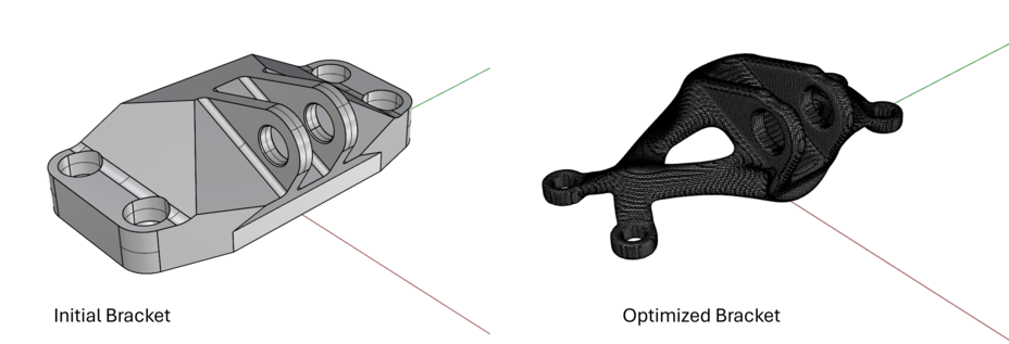
To download the demo files for this workflow download the zip file here.
$ topopt -s "levelopt_bracket.json"
Example: NASA EXCITE Bracket Assembly Optimization
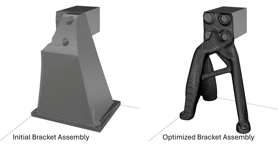
To download the demo files for this workflow download the zip file here.
$ topopt -s "levelopt_NASABracket.json"
Example: Multiple Load Case Drone Optimization
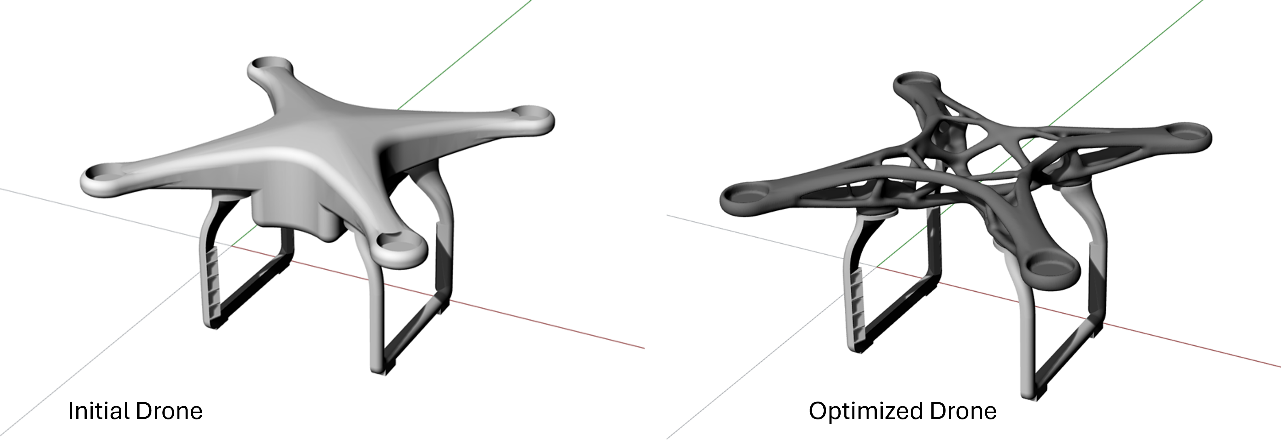
To download the demo files for this workflow download the zip file here.
$ topopt -s "multiload_levelopt_drone.json"
Static Thermal
Static thermal requires the scenario json object to have "type": "StaticThermal".
Materials
All materials need a density value, and can optionally include a "units": member.
Note that all materials will be specified in MKS unless units are specified.
ThermalMaterial
Thermal materials must specify conductivity and specific heat.
A coefficient of thermal expansion can be optionally specified using the expansion_coefficient field.
This example is for steel.
{
  "density": 1200.0,
  "specific_heat": 1100.0,
  "thermal_conductivity": 0.17,
  "type": "Thermal"
}
Boundary Conditions
Fixed
Fixed boundary conditions specify that the boundary is held at a constant temperature and can have a non-zero value.
{
  "boundary": "restraint.stl",
  "type": "fixed",
  "value": 293.15
}
Constant Flux
Specifies a heat flow per unit of surface area.
{
  "boundary": "face.ply",
  "magnitude": 28.0,
  "type": "constant_flux"
}
Convection
Specifies that transfer of heat from a surrounding medium
{
  "boundary": "thermal_plate.ply",
  "coefficient": 525.0,
  "environment_temperature": 343.15,
  "type": "convection"
}
Thermal Metadata
Thermal scenarios have an additional metadata value they must specify.
environment_temperature
The temperature of the surrounding environment.
OpenMP
The intact command line uses OpenMP parallelization.
OpenMP can be controlled by several environment variables.
In general, users will want to specify the number of threads using the OMP_NUM_THREADS environment variable to be
equal to or less than the number of compute cores available.
Logs
Load Balance Check
The Applied Load Matrix summarizes all externally applied loads and the Reaction Force Matrix summarizes reaction forces from supports in a compact and structured format. This matrix helps validate whether the simulation setup obeys global equilibrium — a critical check for simulation correctness.
Matrix Structure
T1 |
T2 |
T3 |
R1 |
R2 |
R3 |
|
|---|---|---|---|---|---|---|
FX |
Fx |
— |
— |
— |
Fx × r₂ |
Fx × r₃ |
FY |
— |
Fy |
— |
Fy × r₁ |
— |
Fy × r₃ |
FZ |
— |
— |
Fz |
Fz × r₁ |
Fz × r₂ |
— |
TOTAL |
∑ |
∑ |
∑ |
∑ |
∑ |
∑ |
T1, T2, T3 → Translational degrees of freedom (forces in X, Y, Z)
R1, R2, R3 → Rotational degrees of freedom (moments about X, Y, Z)
Why Are There Rotational Terms (R1–R3)?
Although only forces are applied in the simulation (all torques are converted to an equivalent force distribution), these forces may be applied at an offset from the reference point (usually the origin). This creates moments via r × F — a cross product of the position vector and the force.
Thus, the R1–R3 columns capture the rotational effects induced by the forces, not explicit moment loads.
Purpose
This matrix allows:
Consistent tracking of applied and reactive loads
Validation that:
Total Applied Load + Total Reaction Force ≈ 0Detection of setup errors like:
Missing constraints
Incorrectly applied loads
Numerical instabilities
Analytics
Intact Solutions gathers anonymous error reports using Sentry.io and anonymous logs using Betterstack.com. You will be notified when installing Intact.Simulation about this data collection.
What is collected?
The collected data include
resolution of simulated model
duration of various steps in the simulation process, such as system assembly, solver setup, solving the linear system
crash dumps
Intact.Simulation does not collect details about your specific model or simulation, nor any personally identifying information.
Why is this data collected?
This data is collected to understand the size of problems that Intact.Simulation is being used on, to understand its performance and bottlenecks to guide future improvements, and to capture information about failures and defects to improve the software’s quality.
Opting out
If you want to opt out, set the environment variable INTACT_NO_ANALYTICS.
For example, using the bash shell, you can do the following to set the environment variable and run Intact.Simulation
INTACT_NO_ANALYTICS=1 ./intact --help
In Windows Powershell, the equivalent command is
$env:INTACT_NO_ANALYTICS=1; .\intact.exe --help